Summary: Linear Equations, Functions, & Quadratic Curves

Comprehensive Lecture Notes, Theoretical Proofs & Graphical Analysis

Published

September 25, 2026

1 Pedagogical Philosophy & Academic Foundations

1.1 Course Prerequisites & Pure Mathematics 1 Standards

A Level Mathematics requires a transition from mechanical computation to deep conceptual fluency. Before progressing through quadratic analysis, students are expected to possess strong proficiency in foundational algebra, including:

Solving linear equations and inequalities.
Solving simultaneous linear equations algebraically and geometrically.
Factoring quadratic expressions over integers.
Manipulating surds and working with exact radical values.

The core textbook for this unit is Pure Mathematics 1 (specifically covering Sections 1.1–1.3, 1.6, and 1.8).

1.2 “Meta-Thinking” vs. Perfunctory Execution

A central tenet of this course is rejecting perfunctory, superficial problem-solving. Students must engage in meta-thinking—actively evaluating the structural rationale behind every mathematical step rather than passively following memorized algorithms.

Every algebraic expression possesses an equivalent geometric representation on the coordinate plane. True mathematical intuition lies in moving fluidly between algebraic manipulation and coordinate geometry.

1.3 Required Homework & Practice Standards

To enforce rigorous learning habits, all assignments must strictly adhere to the following layout and practice standards:

Two-Column Layout:
- Left Column: Formal algebraic derivations, mathematical steps, and precision graph sketches.
- Right Column: Explicit narrative explanations written in full sentences detailing the logical reasoning behind each operation (e.g., explaining why the vertex represents a global minimum or how completing the square isolates the variable).
Elimination of Split Attention: Graphing and derivations must be performed by hand on graph paper with full presence. Reliance on software or secondary materials during live derivations is strictly discouraged.
Peer Verbal Practice: Before each class session, students are required to explain their step-by-step narrative reasoning out loud to a peer to verify conceptual clarity.

2 Linear Relationships & Coordinate Geometry

2.1 Standard Linear Forms and Conversion

A linear relationship between two variables \(x\) and \(y\) represents a constant rate of change. It can be expressed in two primary forms:

Slope-Intercept Form: \(y = mx + c\), where \(m\) is the gradient and \(c\) is the \(y\)-intercept.
General Linear Form: \(ax + by + c = 0\), where \(a, b, c \in \mathbb{R}\).

To understand the geometric properties of the general form, we convert \(ax + by + c = 0\) into slope-intercept form by isolating \(y\):

\[by = -ax - c \implies y = \left(-\frac{a}{b}\right)x - \frac{c}{b}\]

Comparing this directly with \(y = mx + c\) reveals: * Gradient (\(m\)): \(m = -\frac{a}{b}\) * \(y\)-intercept (\(c\)): \(\left(0, -\frac{c}{b}\right)\) * \(x\)-intercept: Setting \(y = 0 \implies ax + c = 0 \implies \left(-\frac{c}{a}, 0\right)\)

2.2 Physical Concept of Gradient (“Rise over Run”)

The gradient \(m\) quantifies the rate of vertical change relative to horizontal change:

\[m = \frac{\text{Rise}}{\text{Run}} = \frac{y_2 - y_1}{x_2 - x_1}\]

Positive Gradient (\(m > 0\)): The line rises from left to right.
Negative Gradient (\(m < 0\)): The line falls from left to right.
Rotational Fulcrum Effect: In \(y = mx + c\), holding \(c\) constant while varying \(m\) rotates the line around the fixed fulcrum point \((0, c)\) on the \(y\)-axis.
Vertical Translation: Holding \(m\) constant while varying \(c\) shifts the line parallel to itself along the \(y\)-axis.

Code

import matplotlib.pyplot as plt
import numpy as np

x = np.linspace(-5, 5, 200)

fig, (ax1, ax2) = plt.subplots(1, 2, figsize=(12, 5))

# Subplot 1: Rotational effect around fulcrum (0,3)
m_values = [-2, -0.5, 0.5, 2]
for m in m_values:
    ax1.plot(x, m * x + 3, label=f'y = {m}x + 3')
ax1.scatter([0], [3], color='red', zorder=5, label='Fulcrum (0, 3)')
ax1.axhline(0, color='black', linewidth=0.8, linestyle='--')
ax1.axvline(0, color='black', linewidth=0.8, linestyle='--')
ax1.set_xlim(-5, 5)
ax1.set_ylim(-5, 10)
ax1.set_title('Gradient Rotation around (0, 3)')
ax1.set_xlabel('x')
ax1.set_ylabel('y')
ax1.grid(True, linestyle=':', alpha=0.6)
ax1.legend()

# Subplot 2: Vertical Translations y = 2x + c
c_values = [-3, 0, 3, 6]
for c in c_values:
    ax2.plot(x, 2 * x + c, label=f'y = 2x + {c}' if c >= 0 else f'y = 2x - {abs(c)}')
ax2.axhline(0, color='black', linewidth=0.8, linestyle='--')
ax2.axvline(0, color='black', linewidth=0.8, linestyle='--')
ax2.set_xlim(-5, 5)
ax2.set_ylim(-8, 12)
ax2.set_title('Vertical Translations y = 2x + c')
ax2.set_xlabel('x')
ax2.set_ylabel('y')
ax2.grid(True, linestyle=':', alpha=0.6)
ax2.legend()

plt.tight_layout()
plt.show()

Figure 1: Rotational effect of gradient m around the fulcrum (0,3) and vertical translation of linear graphs.

2.3 The Universal Intercept Method for Linear Graphs

Because two points uniquely determine a straight line, the most efficient plotting strategy is identifying the axis intercepts:

\(y\)-intercept: Set \(x = 0 \implies\) solve for \(y\).
\(x\)-intercept: Set \(y = 0 \implies\) solve for \(x\).

2.3.1 Worked Example

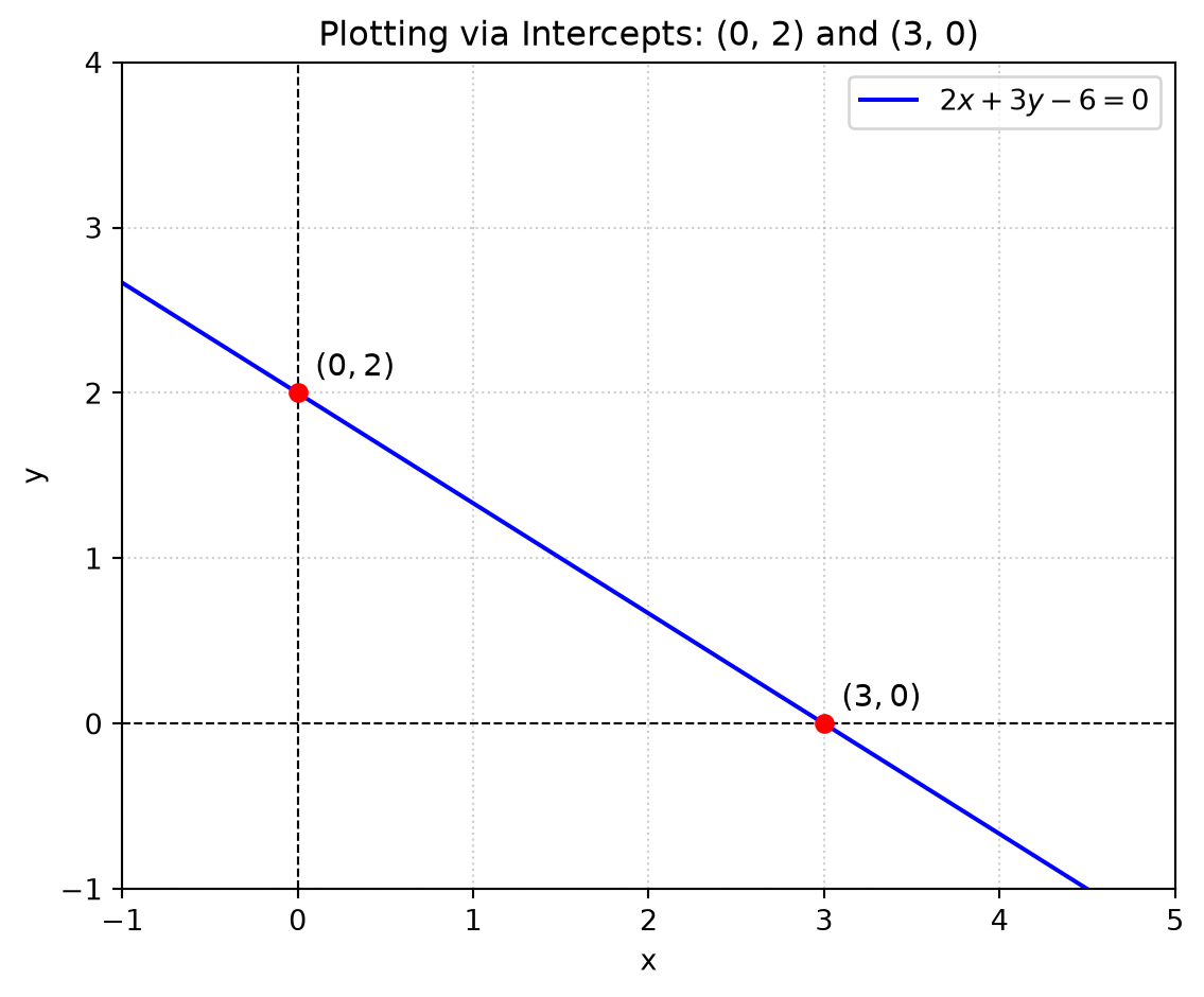
Plot the line \(2x + 3y - 6 = 0\): * Set \(x = 0 \implies 3y = 6 \implies y = 2 \implies (0, 2)\) * Set \(y = 0 \implies 2x = 6 \implies x = 3 \implies (3, 0)\)

Code

plt.figure(figsize=(6, 5))
x = np.linspace(-2, 5, 200)
y = (6 - 2 * x) / 3

plt.plot(x, y, color='blue', label='$2x + 3y - 6 = 0$')
plt.scatter([0, 3], [2, 0], color='red', zorder=5)
plt.annotate('$(0, 2)$', (0.1, 2.1), fontsize=11, fontweight='bold')
plt.annotate('$(3, 0)$', (3.1, 0.1), fontsize=11, fontweight='bold')

plt.axhline(0, color='black', linewidth=0.8, linestyle='--')
plt.axvline(0, color='black', linewidth=0.8, linestyle='--')
plt.xlim(-1, 5)
plt.ylim(-1, 4)
plt.xlabel('x')
plt.ylabel('y')
plt.title('Plotting via Intercepts: (0, 2) and (3, 0)')
plt.grid(True, linestyle=':', alpha=0.6)
plt.legend()
plt.tight_layout()
plt.show()

Figure 2: The Intercept Method applied to 2x + 3y - 6 = 0.

2.4 Systems of Linear Equations & Geometric Classifications

An algebraic system of two linear equations corresponds to the geometric relationship between two lines in a plane:

Parallel Lines: Equal gradients (\(m_1 = m_2\)) but distinct \(y\)-intercepts (\(c_1 \neq c_2\)). The lines never intersect \(\implies\) No solution.
Intersecting Lines: Different gradients (\(m_1 \neq m_2\)). The lines intersect at a single point \((x_0, y_0)\) \(\implies\) 1 Unique solution.
Coincident Lines: Equal gradients (\(m_1 = m_2\)) and identical \(y\)-intercepts (\(c_1 = c_2\)). The lines overlap entirely \(\implies\) Infinitely many solutions.

3 Universal Function Graphing Strategy & Non-Linear Curves

3.1 Definition of a Function \(y = f(x)\)

A function \(y = f(x)\) expresses an explicit mathematical rule where each input \(x\) maps to a unique output \(y\).

3.2 The Universal Intercept Protocol

For any function \(y = f(x)\)—whether linear, quadratic, circular, or cubic—identifying key landmarks begins with the Universal Intercept Protocol:

\(y\)-intercept: Evaluate \(y = f(0)\) by setting \(x = 0\).
\(x\)-intercept(s): Solve \(f(x) = 0\) by setting \(y = 0\).

3.3 Demonstration on Non-Linear Curves

3.3.1 Circular Curve (\(y^2 = 4 - x^2 \iff x^2 + y^2 = 4\))

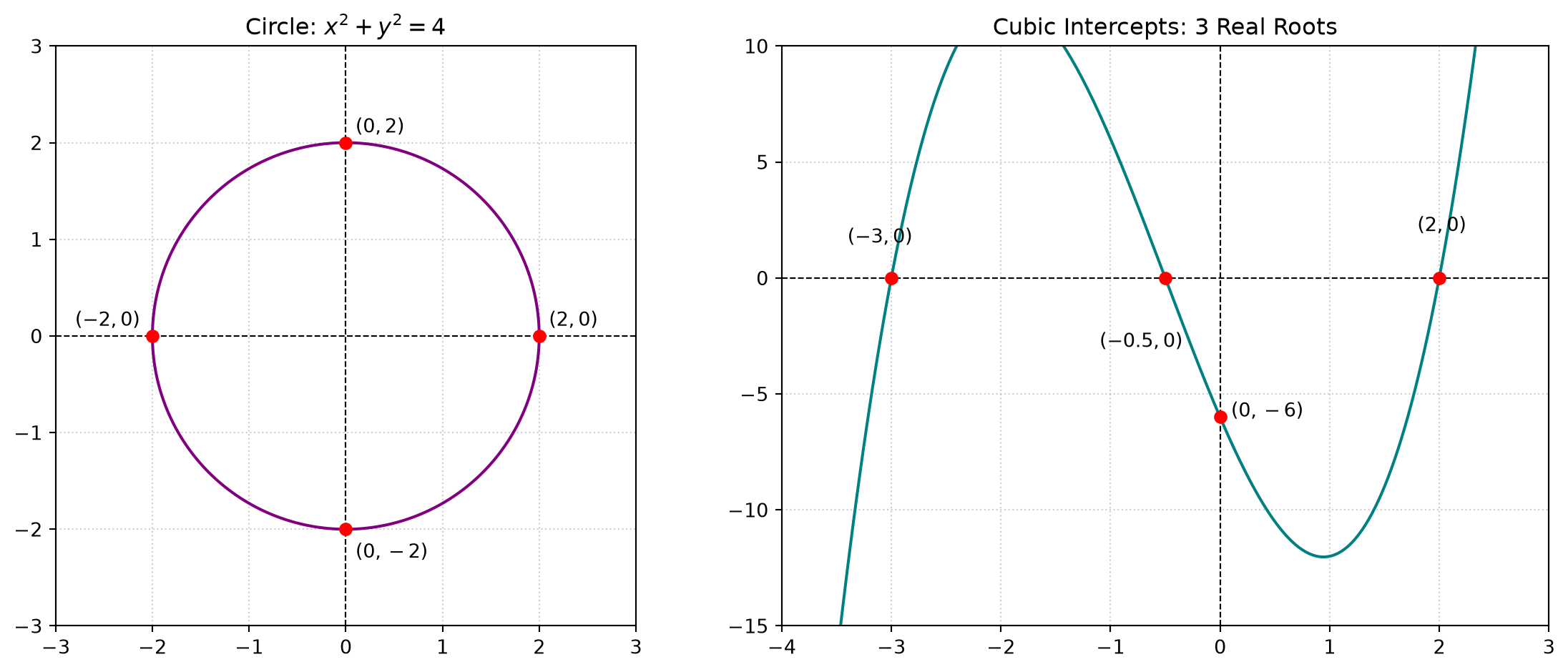
Applying the protocol to \(y^2 = 4 - x^2\): * \(y\)-intercepts: Set \(x = 0 \implies y^2 = 4 \implies y = \pm 2 \implies (0, 2) \text{ and } (0, -2)\). * \(x\)-intercepts: Set \(y = 0 \implies x^2 = 4 \implies x = \pm 2 \implies (2, 0) \text{ and } (-2, 0)\).

Connecting these four symmetric points yields a circle centered at \((0,0)\) with radius \(r = 2\).

3.3.2 Higher-Order Polynomials

For a cubic function such as \(y = (x - 2)(2x^2 + 7x + 3)\): * \(y\)-intercept: Set \(x = 0 \implies y = (-2)(3) = -6 \implies (0, -6)\). * \(x\)-intercepts: Set \(y = 0 \implies (x - 2)(2x + 1)(x + 3) = 0 \implies x = 2, x = -0.5, x = -3\). * The curve crosses the \(x\)-axis at three distinct points.

Code

fig, (ax1, ax2) = plt.subplots(1, 2, figsize=(12, 5))

# Circle x^2 + y^2 = 4
theta = np.linspace(0, 2*np.pi, 300)
ax1.plot(2 * np.cos(theta), 2 * np.sin(theta), color='purple', label='$x^2 + y^2 = 4$')
ax1.scatter([0, 0, 2, -2], [2, -2, 0, 0], color='red', zorder=5)
ax1.annotate('$(0, 2)$', (0.1, 2.1))
ax1.annotate('$(0, -2)$', (0.1, -2.3))
ax1.annotate('$(2, 0)$', (2.1, 0.1))
ax1.annotate('$(-2, 0)$', (-2.8, 0.1))
ax1.axhline(0, color='black', linewidth=0.8, linestyle='--')
ax1.axvline(0, color='black', linewidth=0.8, linestyle='--')
ax1.set_aspect('equal')
ax1.set_xlim(-3, 3)
ax1.set_ylim(-3, 3)
ax1.set_title('Circle: $x^2 + y^2 = 4$')
ax1.grid(True, linestyle=':', alpha=0.6)

# Cubic Polynomial y = (x - 2)(2x^2 + 7x + 3)
x_cubic = np.linspace(-3.5, 2.5, 200)
y_cubic = (x_cubic - 2) * (2 * x_cubic**2 + 7 * x_cubic + 3)
ax2.plot(x_cubic, y_cubic, color='teal', label='$y = (x-2)(2x^2+7x+3)$')
ax2.scatter([-3, -0.5, 2, 0], [0, 0, 0, -6], color='red', zorder=5)
ax2.annotate('$(-3, 0)$', (-3.4, 1.5))
ax2.annotate('$(-0.5, 0)$', (-1.1, -3))
ax2.annotate('$(2, 0)$', (1.8, 2))
ax2.annotate('$(0, -6)$', (0.1, -6))
ax2.axhline(0, color='black', linewidth=0.8, linestyle='--')
ax2.axvline(0, color='black', linewidth=0.8, linestyle='--')
ax2.set_xlim(-4, 3)
ax2.set_ylim(-15, 10)
ax2.set_title('Cubic Intercepts: 3 Real Roots')
ax2.grid(True, linestyle=':', alpha=0.6)

plt.tight_layout()
plt.show()

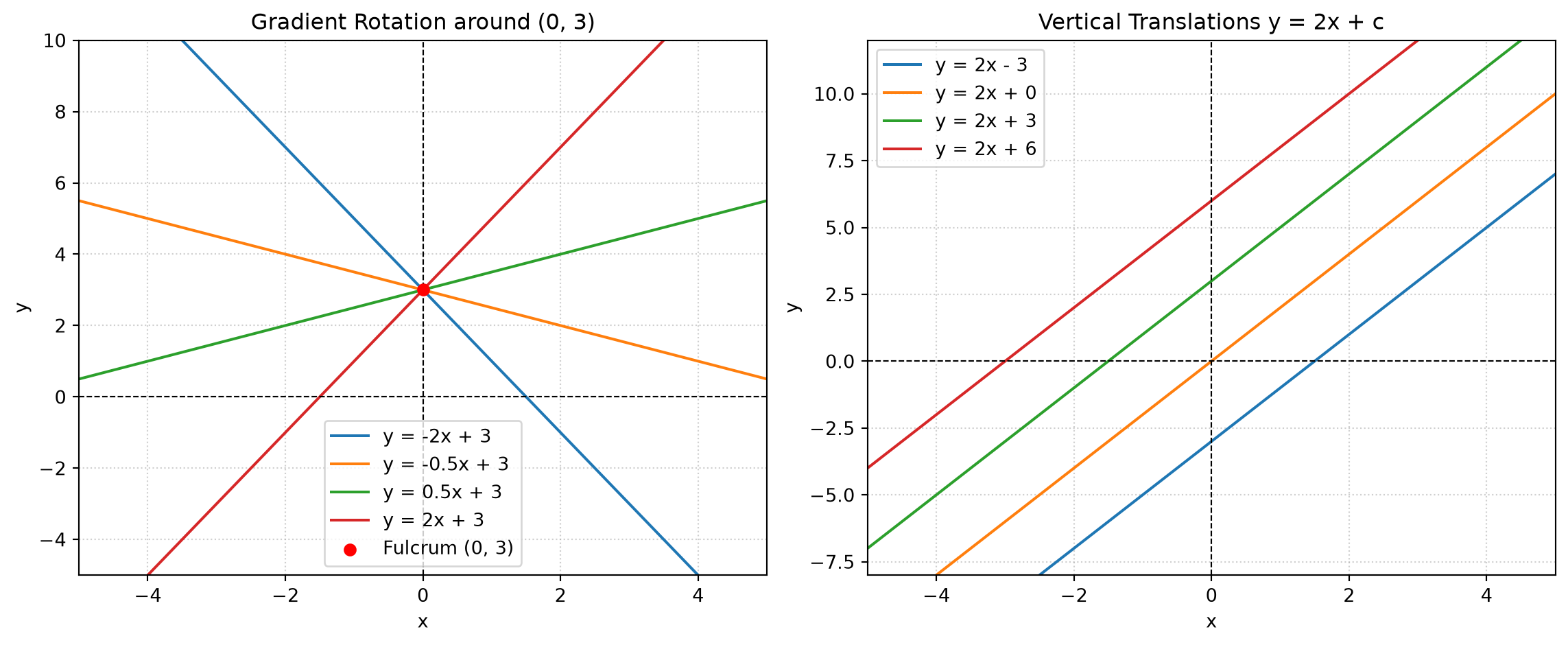
Figure 3: Universal Intercept Protocol applied to a circle (x² + y² = 4) and a cubic polynomial.

4 Fundamentals of Quadratic Curves & Parabolas

4.1 Properties of the Standard Parabola (\(y = x^2\))

Non-Negativity: For all \(x \in \mathbb{R}\), \(x^2 \ge 0\), meaning \(y\) cannot be negative.
Symmetry: \(f(-x) = (-x)^2 = x^2 = f(x)\), making the curve perfectly symmetrical across the \(y\)-axis (\(x = 0\)).
Vertex: The lowest turning point sits at the origin \((0,0)\), acting as a global minimum.

4.2 The Scaling Coefficient \(a\) in \(y = ax^2\)

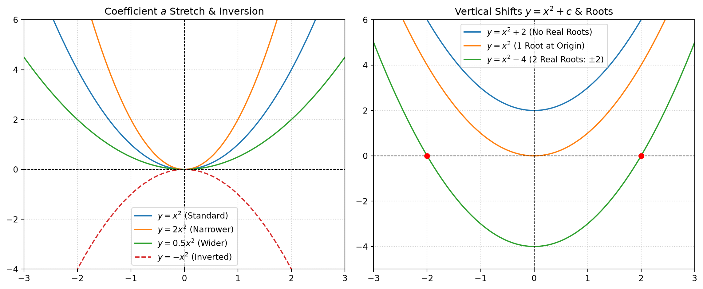
The coefficient \(a\) dictates the vertical stretch/compression and direction of opening: * \(|a| > 1\): Vertically stretches the parabola, making it narrower. * \(0 < |a| < 1\): Vertically compresses the parabola, making it wider. * \(a > 0\): Opens upward (minimum turning point). * \(a < 0\): Opens downward (maximum turning point).

4.3 Vertical Translations (\(y = ax^2 + c\))

The constant \(c\) translates the parabola vertically along the \(y\)-axis by \(c\) units, shifting the vertex to \((0, c)\).

Code

fig, (ax1, ax2) = plt.subplots(1, 2, figsize=(12, 5))

x = np.linspace(-3, 3, 200)

# Subplot 1: Effect of coefficient a
ax1.plot(x, x**2, label='$y = x^2$ (Standard)')
ax1.plot(x, 2 * x**2, label='$y = 2x^2$ (Narrower)')
ax1.plot(x, 0.5 * x**2, label='$y = 0.5x^2$ (Wider)')
ax1.plot(x, -x**2, label='$y = -x^2$ (Inverted)', linestyle='--')
ax1.axhline(0, color='black', linewidth=0.8, linestyle='--')
ax1.axvline(0, color='black', linewidth=0.8, linestyle='--')
ax1.set_xlim(-3, 3)
ax1.set_ylim(-4, 6)
ax1.set_title('Coefficient $a$ Stretch & Inversion')
ax1.grid(True, linestyle=':', alpha=0.6)
ax1.legend()

# Subplot 2: Vertical translations y = x^2 + c
ax2.plot(x, x**2 + 2, label='$y = x^2 + 2$ (No Real Roots)')
ax2.plot(x, x**2, label='$y = x^2$ (1 Root at Origin)')
ax2.plot(x, x**2 - 4, label='$y = x^2 - 4$ (2 Real Roots: $\\pm 2$)')
ax2.scatter([2, -2], [0, 0], color='red', zorder=5)
ax2.axhline(0, color='black', linewidth=0.8, linestyle='--')
ax2.axvline(0, color='black', linewidth=0.8, linestyle='--')
ax2.set_xlim(-3, 3)
ax2.set_ylim(-5, 6)
ax2.set_title('Vertical Shifts $y = x^2 + c$ & Roots')
ax2.grid(True, linestyle=':', alpha=0.6)
ax2.legend()

plt.tight_layout()
plt.show()

Figure 4: Effects of scaling coefficient a and vertical translation c on parabolas.

5 Advanced Quadratic Forms, Vertex Derivation & Symmetry

5.1 Derivation of Vertex Formulas for \(y = ax^2 + bx\)

To analyze \(y = ax^2 + bx\), we factorize the expression to locate its \(x\)-intercepts:

\[y = ax\left(x + \frac{b}{a}\right)\]

\(y\)-intercept: Set \(x = 0 \implies y = 0 \implies (0,0)\).
\(x\)-intercepts: Set \(y = 0 \implies ax\left(x + \frac{b}{a}\right) = 0 \implies x_1 = 0 \quad \text{and} \quad x_2 = -\frac{b}{a}\).
Axis of Symmetry (\(x_v\)): Due to parabolic symmetry, the vertex \(x\)-coordinate lies at the exact midpoint of the two \(x\)-intercepts: \[x_v = \frac{0 + \left(-\frac{b}{a}\right)}{2} = -\frac{b}{2a}\]
Vertex \(y\)-coordinate (\(y_v\)): Substitute \(x_v = -\frac{b}{2a}\) back into the equation: \[y_v = a\left(-\frac{b}{2a}\right)^2 + b\left(-\frac{b}{2a}\right) = a\left(\frac{b^2}{4a^2}\right) - \frac{b^2}{2a} = \frac{b^2}{4a} - \frac{b^2}{2a} = -\frac{b^2}{4a}\]

\[\text{Vertex Coordinates: } \mathbf{\left(-\frac{b}{2a}, -\frac{b^2}{4a}\right)}\]

5.1.1 Worked Example: \(y = 2x^2 + 6x\)

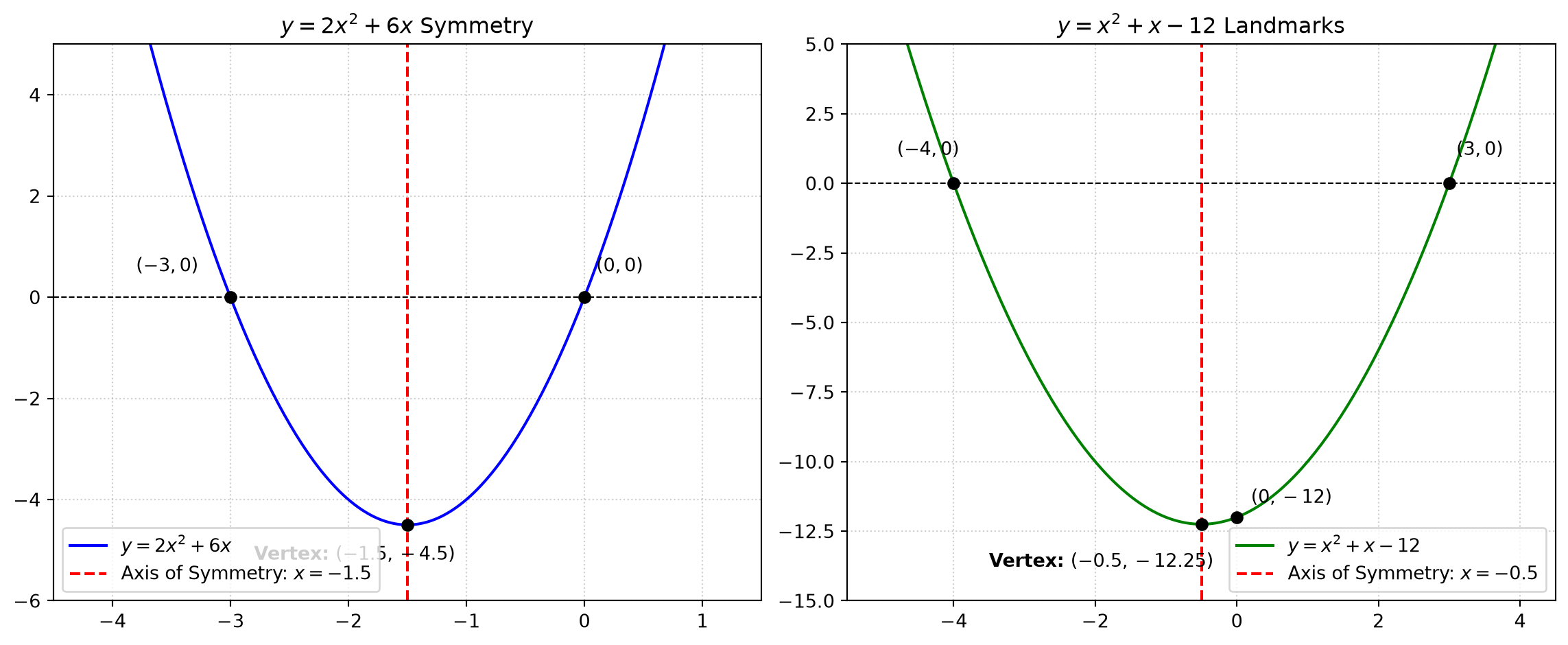
\(x\)-intercepts: \(2x(x + 3) = 0 \implies (0,0) \text{ and } (-3,0)\).
Axis of Symmetry: \(x_v = \frac{0 + (-3)}{2} = -1.5\).
Vertex \(y\)-value: \(y_v = 2(-1.5)^2 + 6(-1.5) = 4.5 - 9 = -4.5\).
Vertex: \((-1.5, -4.5)\).

5.2 General Quadratic Form \(y = ax^2 + bx + c\)

Adding \(c\) translates the parabola \(y = ax^2 + bx\) vertically by \(c\) units: * \(y\)-intercept: Set \(x = 0 \implies y = c \implies (0, c)\). * Axis of Symmetry: Substituting \(y = c \implies ax^2 + bx + c = c \implies ax^2 + bx = 0 \implies x = 0 \text{ and } x = -\frac{b}{a}\). The midpoint remains \(x_v = -\frac{b}{2a}\).

5.2.1 Factorizable Example: \(y = x^2 + x - 12\)

Factorize: \(y = (x - 3)(x + 4)\).
\(y\)-intercept: Set \(x = 0 \implies y = -12 \implies (0, -12)\).
\(x\)-intercepts: Set \(y = 0 \implies (x - 3)(x + 4) = 0 \implies (3,0) \text{ and } (-4,0)\).
Vertex \(x\)-coordinate: \(x_v = \frac{3 + (-4)}{2} = -0.5\).
Vertex \(y\)-coordinate: \(y_v = (-0.5 - 3)(-0.5 + 4) = (-3.5)(3.5) = -12.25\).
Vertex: \((-0.5, -12.25)\).

5.3 Uniqueness of the Vertex

The vertex is geometrically unique: it is the only point on a parabola that possesses a single unique \(x\)-value for its \(y\)-value. For every other \(y\)-value above (or below) the vertex, there exist exactly two symmetric \(x\)-values equidistant from the axis of symmetry \(x = -\frac{b}{2a}\).

Code

fig, (ax1, ax2) = plt.subplots(1, 2, figsize=(12, 5))

# Plot 1: y = 2x^2 + 6x
x1 = np.linspace(-4, 1, 200)
y1 = 2 * x1**2 + 6 * x1
ax1.plot(x1, y1, color='blue', label='$y = 2x^2 + 6x$')
ax1.axvline(-1.5, color='red', linestyle='--', label='Axis of Symmetry: $x = -1.5$')
ax1.scatter([0, -3, -1.5], [0, 0, -4.5], color='black', zorder=5)
ax1.annotate('$(0,0)$', (0.1, 0.5))
ax1.annotate('$(-3,0)$', (-3.8, 0.5))
ax1.annotate('Vertex: $(-1.5, -4.5)$', (-2.8, -5.2), fontweight='bold')
ax1.axhline(0, color='black', linewidth=0.8, linestyle='--')
ax1.set_xlim(-4.5, 1.5)
ax1.set_ylim(-6, 5)
ax1.set_title('$y = 2x^2 + 6x$ Symmetry')
ax1.grid(True, linestyle=':', alpha=0.6)
ax1.legend()

# Plot 2: y = x^2 + x - 12
x2 = np.linspace(-5, 4, 200)
y2 = x2**2 + x2 - 12
ax2.plot(x2, y2, color='green', label='$y = x^2 + x - 12$')
ax2.axvline(-0.5, color='red', linestyle='--', label='Axis of Symmetry: $x = -0.5$')
ax2.scatter([3, -4, 0, -0.5], [0, 0, -12, -12.25], color='black', zorder=5)
ax2.annotate('$(3,0)$', (3.1, 1))
ax2.annotate('$(-4,0)$', (-4.8, 1))
ax2.annotate('$(0,-12)$', (0.2, -11.5))
ax2.annotate('Vertex: $(-0.5, -12.25)$', (-3.5, -13.8), fontweight='bold')
ax2.axhline(0, color='black', linewidth=0.8, linestyle='--')
ax2.set_xlim(-5.5, 4.5)
ax2.set_ylim(-15, 5)
ax2.set_title('$y = x^2 + x - 12$ Landmarks')
ax2.grid(True, linestyle=':', alpha=0.6)
ax2.legend()

plt.tight_layout()
plt.show()

Figure 5: Parabolic symmetry, axis of symmetry, and vertex for y = 2x² + 6x and y = x² + x - 12.

6 Completing the Square, Formal Proof, & The Discriminant

6.1 Completing the Square Technique

When a quadratic expression cannot be easily factorized over integers, we isolate \(x\) by transforming the quadratic into a perfect square binomial:

\[(x + a)^2 = x^2 + 2ax + a^2\]

6.1.1 Numerical Example: Solve \(x^2 + x - 7 = 0\)

Group the \(x\)-terms: \((x^2 + x) - 7 = 0\).
Take half the linear coefficient \(\left(\frac{1}{2}\right)\) and square it \(\left(\frac{1}{4}\right)\). Add and subtract inside the expression: \[\left(x^2 + x + \frac{1}{4}\right) - \frac{1}{4} - 7 = 0\]
Write as a perfect square: \[\left(x + \frac{1}{2}\right)^2 - \frac{29}{4} = 0 \implies \left(x + \frac{1}{2}\right)^2 = \frac{29}{4}\]
Take the square root on both sides: \[x + \frac{1}{2} = \pm \frac{\sqrt{29}}{2} \implies x = -\frac{1}{2} \pm \frac{\sqrt{29}}{2}\]

6.2 General Proof of the Quadratic Formula

Starting with the general quadratic equation \(ax^2 + bx + c = 0\) (where \(a \neq 0\)):

\[\text{Divide by } a: \quad x^2 + \frac{b}{a}x + \frac{c}{a} = 0\]

Rewrite the middle linear term as \(2 \cdot \left(\frac{b}{2a}\right)x\) and complete the square by adding and subtracting \(\left(\frac{b}{2a}\right)^2\):

\[\left[x^2 + 2\left(\frac{b}{2a}\right)x + \left(\frac{b}{2a}\right)^2\right] - \left(\frac{b}{2a}\right)^2 + \frac{c}{a} = 0\]

\[\left(x + \frac{b}{2a}\right)^2 - \frac{b^2}{4a^2} + \frac{c}{a} = 0\]

\[\left(x + \frac{b}{2a}\right)^2 = \frac{b^2}{4a^2} - \frac{c}{a} = \frac{b^2 - 4ac}{4a^2}\]

Taking the square root on both sides:

\[x + \frac{b}{2a} = \pm \sqrt{\frac{b^2 - 4ac}{4a^2}} = \pm \frac{\sqrt{b^2 - 4ac}}{2a}\]

\[\mathbf{x = \frac{-b \pm \sqrt{b^2 - 4ac}}{2a}}\]

6.2.1 Structural & Geometric Interpretation of the Formula

The quadratic formula is composed of two geometric components: 1. Axis of Symmetry: The term \(-\frac{b}{2a}\) gives the horizontal center line of the parabola. 2. Symmetric Offset: The term \(\pm \frac{\sqrt{b^2 - 4ac}}{2a}\) gives the exact horizontal distance from the axis of symmetry to the two \(x\)-intercepts.

\[\text{Root } x_1, x_2 = \underbrace{-\frac{b}{2a}}_{\text{Axis of Symmetry}} \pm \underbrace{\frac{\sqrt{b^2 - 4ac}}{2a}}_{\text{Distance to Intercepts}}\]

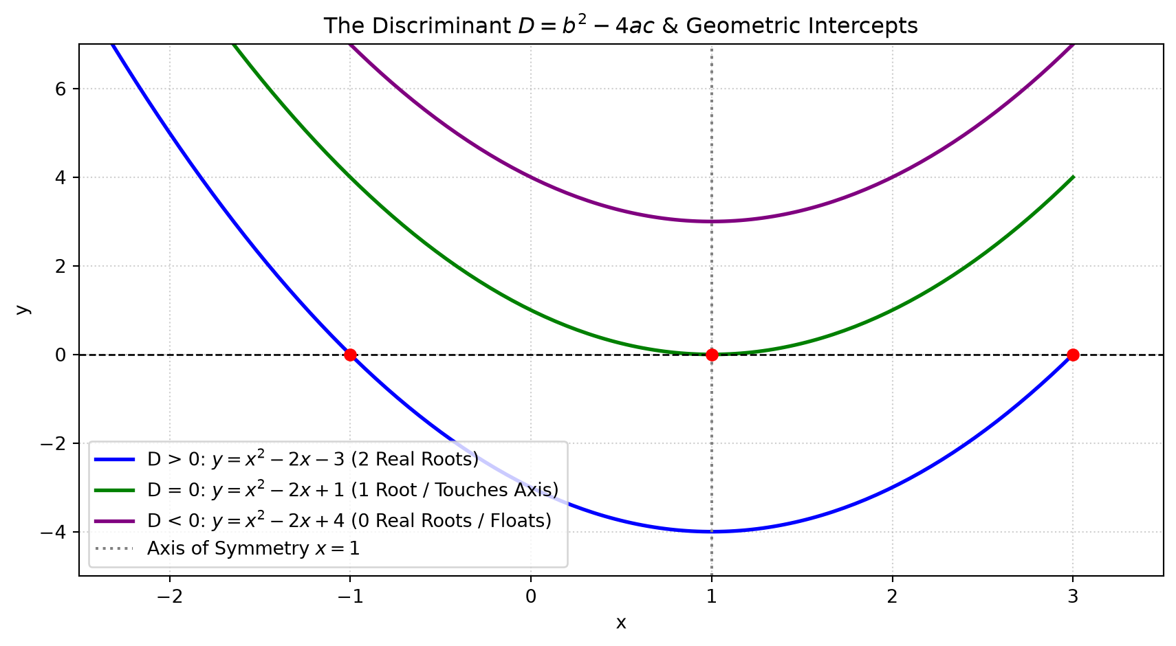
6.3 The Discriminant (\(D = b^2 - 4ac\))

The expression under the radical sign, \(D = b^2 - 4ac\), determines the nature and number of real roots (and \(x\)-intercepts):

\(b^2 - 4ac > 0\): 2 Distinct Real Roots. The parabola intersects the \(x\)-axis at two distinct points equidistant from \(x = -\frac{b}{2a}\).
\(b^2 - 4ac = 0\): 1 Repeated Real Root. The offset distance is zero, meaning the vertex sits directly on the \(x\)-axis at \(x = -\frac{b}{2a}\).
\(b^2 - 4ac < 0\): No Real Roots. The square root of a negative number is non-real, meaning the parabola floats entirely above (if \(a > 0\)) or lies entirely below (if \(a < 0\)) the \(x\)-axis without touching it.

Code

plt.figure(figsize=(9, 5))
x = np.linspace(-3, 3, 200)

plt.plot(x, x**2 - 2*x - 3, color='blue', linewidth=2, label='D > 0: $y = x^2 - 2x - 3$ (2 Real Roots)')
plt.plot(x, x**2 - 2*x + 1, color='green', linewidth=2, label='D = 0: $y = x^2 - 2x + 1$ (1 Root / Touches Axis)')
plt.plot(x, x**2 - 2*x + 4, color='purple', linewidth=2, label='D < 0: $y = x^2 - 2x + 4$ (0 Real Roots / Floats)')

plt.scatter([3, -1, 1], [0, 0, 0], color='red', zorder=5)
plt.axhline(0, color='black', linewidth=1, linestyle='--')
plt.axvline(1, color='gray', linestyle=':', label='Axis of Symmetry $x = 1$')

plt.xlim(-2.5, 3.5)
plt.ylim(-5, 7)
plt.xlabel('x')
plt.ylabel('y')
plt.title('The Discriminant $D = b^2 - 4ac$ & Geometric Intercepts')
plt.grid(True, linestyle=':', alpha=0.6)
plt.legend()
plt.tight_layout()
plt.show()

Figure 6: Geometric classification of parabolas based on the Discriminant D = b² - 4ac.

7 Critical Graphing Protocol & Homework Assignment

7.1 Master Checklist for Sketching Any Parabola

When sketching a quadratic curve \(y = ax^2 + bx + c\), identify and label these four landmarks:

\(y\)-intercept: Evaluate \((0, c)\).
Discriminant Check & \(x\)-intercepts: Compute \(D = b^2 - 4ac\). If \(D \ge 0\), solve for roots via factoring or the quadratic formula.
Axis of Symmetry: Draw the dashed line \(x = -\frac{b}{2a}\).
Vertex Coordinates: Calculate \(\left(-\frac{b}{2a}, \frac{4ac - b^2}{4a}\right)\).

7.2 Homework Exercises & Textbook Reference

Textbook: Pure Mathematics 1 (Sections 1.1–1.3, 1.6, and 1.8).
Exercises: Complete selected sub-questions from Exercises 1A, 1B, and 1C using the mandatory two-column layout.
Practice Task: Reproduce the algebraic proof of the quadratic formula via completing the square on a blank page without looking at notes, and practice verbally presenting the proof to a peer.