Solving a quadratic equation and a simultaneous linear equation is equivalent to finding the points of intersection of a quadratic curve and a straight line. This is a fundamental concept in A-Level Mathematics, bridging algebra and geometry.
1. Intersection of Two Linear Equations
As we explored in earlier sessions, a linear equation y = mx + c represents a straight line. When we have two such equations: 1. y = m_1x + c_1 2. y = m_2x + c_2
Solving them “simultaneously” means finding a point (x, y) that lies on both lines. Algebraically, we equate the two expressions for y:
m_1x + c_1 = m_2x + c_2
This simplifies to a single linear equation in x: (m_1 - m_2)x = c_2 - c_1
Example: Finding the intersection
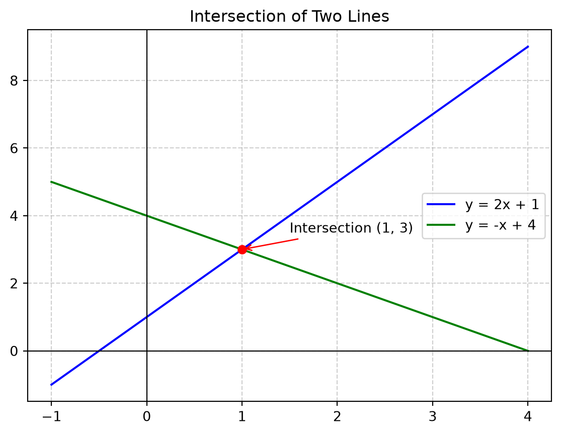
Consider the lines y = 2x + 1 and y = -x + 4. Equating them: 2x + 1 = -x + 43x = 3 \implies x = 1 Substituting x=1 into y = 2x + 1 gives y = 2(1) + 1 = 3. The point of intersection is (1, 3).
The same concept of “simultaneous equations” extends to curves. If we have a quadratic curve y = ax^2 + bx + c and a straight line y = mx + k, the points where they intersect must satisfy both equations.
To find these points, we set the quadratic equal to the linear: ax^2 + bx + c = mx + k
Rearranging into standard quadratic form (Ax^2 + Bx + C = 0): ax^2 + (b-m)x + (c-k) = 0
The solutions to this equation are the x-coordinates of the intersection points.
3. Geometric Interpretation and the Discriminant
The number of solutions to the resulting quadratic equation determines how the line and curve relate geometrically. This is governed by the discriminant\Delta = B^2 - 4AC of the combined equation.
Discriminant
Number of Solutions
Geometric Relationship
\Delta > 0
2 distinct real roots
The line cuts the curve at two points.
\Delta = 0
1 repeated real root
The line is a tangent to the curve.
\Delta < 0
No real roots
The line does not meet the curve.
Case 1: Two Points of Intersection (\Delta > 0)
Find the points of intersection of y = x^2 - 4x + 3 and y = x - 1.
Algebraic Solution:x^2 - 4x + 3 = x - 1x^2 - 5x + 4 = 0(x - 1)(x - 4) = 0 \implies x = 1, x = 4 For x=1, y = 1 - 1 = 0. For x=4, y = 4 - 1 = 3. Points: (1, 0) and (4, 3).
Case 2: One Point of Intersection - Tangent (\Delta = 0)
Find the point of intersection of y = x^2 - 2x + 5 and y = 2x + 1.
Algebraic Solution:x^2 - 2x + 5 = 2x + 1x^2 - 4x + 4 = 0(x - 2)^2 = 0 \implies x = 2 For x=2, y = 2(2) + 1 = 5. Point: (2, 5). Since there is only one solution, the line is a tangent.
Case 3: No Intersection (\Delta < 0)
Show that y = x^2 + 1 and y = x - 2 do not intersect.
Algebraic Solution:x^2 + 1 = x - 2x^2 - x + 3 = 0 Discriminant \Delta = (-1)^2 - 4(1)(3) = 1 - 12 = -11. Since \Delta < 0, there are no real solutions, and the line never meets the curve.
4. Visualizing the Three Cases
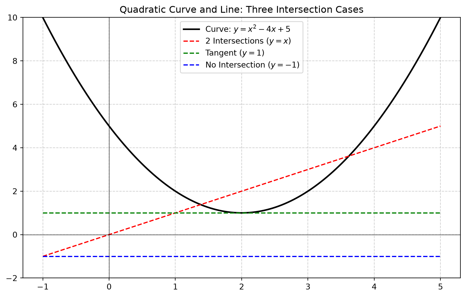
The following graph illustrates how different lines can interact with the same quadratic curve y = x^2 - 4x + 5.
Code
import numpy as npimport matplotlib.pyplot as pltx = np.linspace(-1, 5, 400)y_curve = x**2-4*x +5# Vertex at (2, 1)# Line 1: y = x (Two intersections)y1 = x # x^2 - 4x + 5 = x => x^2 - 5x + 5 = 0. delta = 25 - 20 = 5 > 0# Line 2: y = 1 (Tangent at the vertex)y2 =0*x +1# x^2 - 4x + 5 = 1 => x^2 - 4x + 4 = 0. delta = 16 - 16 = 0# Line 3: y = -1 (No intersection)y3 =0*x -1# x^2 - 4x + 5 = -1 => x^2 - 4x + 6 = 0. delta = 16 - 24 = -8 < 0plt.figure(figsize=(10, 6))plt.plot(x, y_curve, 'k', linewidth=2, label='Curve: $y = x^2 - 4x + 5$')plt.plot(x, y1, 'r--', label='2 Intersections ($y = x$)')plt.plot(x, y2, 'g--', label='Tangent ($y = 1$)')plt.plot(x, y3, 'b--', label='No Intersection ($y = -1$)')plt.axhline(0, color='black', linewidth=0.5)plt.axvline(0, color='black', linewidth=0.5)plt.ylim(-2, 10)plt.grid(True, linestyle='--', alpha=0.6)plt.legend()plt.title('Quadratic Curve and Line: Three Intersection Cases')plt.show()
Summary of the Procedure
Set up: Write both equations in the form y = f(x).
Equate: Set f(x)_{quadratic} = f(x)_{linear}.
Solve: Rearrange into Ax^2 + Bx + C = 0 and solve for x.
Find y: Substitute the x-values into the linear equation (it’s usually easier).
Conditions: If a problem asks for the “condition” for a line to be a tangent or not intersect, use the discriminant \Delta on the combined equation.