Elasticities of Demand, Decision Mechanics, and Case Studies

Published

September 24, 2026

1 Introduction to Elasticity of Demand

Elasticity is a general measure of the responsiveness of one variable to changes in another variable, ceteris paribus (all other things remaining equal). Because elasticity measures relative or percentage changes, it is expressed as a unitless coefficient or pure ratio, meaning original measurement units cancel out.

2 Elasticities of Demand: Theory and Mathematical Representations

2.1 Price Elasticity of Demand (PED)

2.1.1 Definition and Formula

Price Elasticity of Demand ($\text{PED}$) measures the responsiveness of the quantity demanded of a product following a change in its own price.

\[\text{PED} = \frac{\% \Delta Q_d}{\% \Delta P} = \frac{\frac{\Delta Q}{Q_1} \times 100}{\frac{\Delta P}{P_1} \times 100} = \frac{\Delta Q}{\Delta P} \times \frac{P_1}{Q_1}\]

By the Law of Demand, price and quantity demanded move in opposite directions, making the default mathematical value of $\text{PED}$ negative. However, standard economic convention drops the negative sign and treats $\text{PED}$ in absolute terms.

2.1.2 Behavior Along a Downward-Sloping Linear Demand Curve

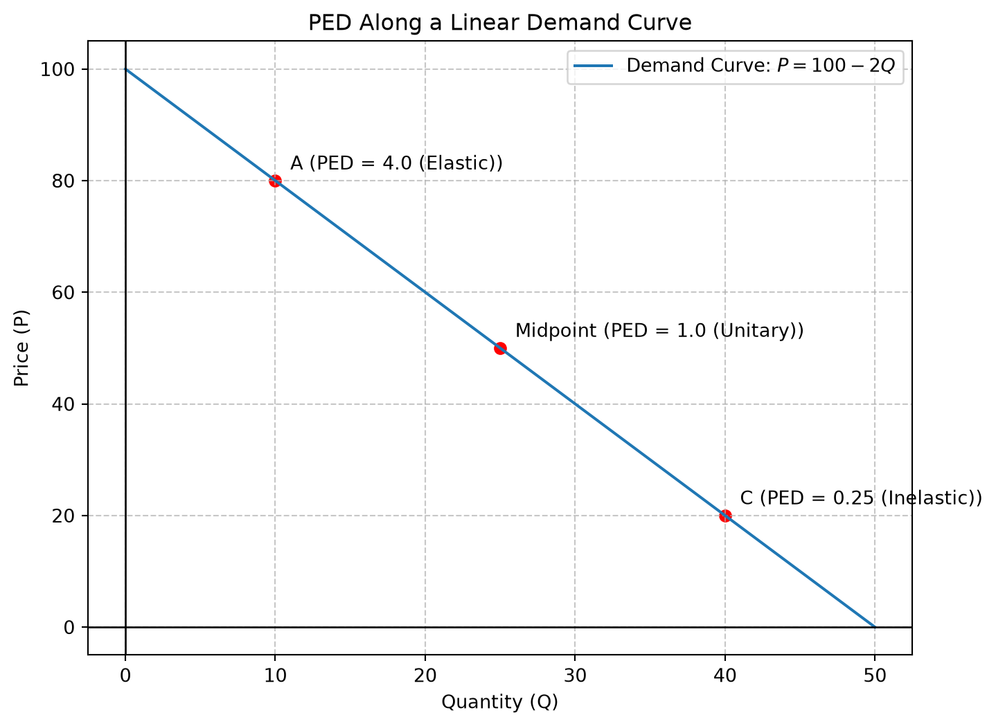
Along a linear downward-sloping demand curve ($P = a - bQ$), the slope or gradient ($\frac{\Delta P}{\Delta Q} = -b$) remains constant throughout. However, $\text{PED}$ does not remain constant along the curve because it depends on the ratio of absolute price to quantity ($\frac{P}{Q}$):

\[\text{PED} = \left( \frac{\Delta Q}{\Delta P} \right) \times \left( \frac{P}{Q} \right) = \left( \frac{1}{\text{Slope}} \right) \times \left( \frac{P}{Q} \right)\]

Upper Segment (High Price, Low Quantity): The ratio $\frac{P}{Q}$ is large, making $\text{PED} > 1$ (Price Elastic). Small price changes trigger proportionately larger percentage changes in quantity demanded.
Midpoint ($P = \frac{a}{2}, Q = \frac{a}{2b}$): The term $\frac{\Delta Q}{\Delta P}$ and the ratio $\frac{P}{Q}$ become exact mathematical reciprocals ($\frac{\Delta Q}{\Delta P} = \frac{Q}{P}$), yielding $\text{PED} = 1.0$ (Unitary Elastic).
Lower Segment (Low Price, High Quantity): The ratio $\frac{P}{Q}$ is small, making $\text{PED} < 1$ (Price Inelastic). Large price changes yield proportionately smaller percentage changes in quantity demanded.

Numerical Class Example

Given the demand function: \[P = 100 - 2Q \implies Q = 50 - 0.5P\]

The slope derivative $\frac{dQ}{dP} = -0.5$ is constant. Using the formula $\text{PED} = \left| \frac{dQ}{dP} \times \frac{P}{Q} \right|$:

Point	Price ($P$)	Quantity ($Q$)	Calculation	$\text{PED}$ Value	Classification
A	80	10	$\left\| -0.5 \times \frac{80}{10} \right\|$	4.0	Price Elastic
Midpoint	50	25	$\left\| -0.5 \times \frac{50}{25} \right\|$	1.0	Unitary Elastic
C	20	40	$\left\| -0.5 \times \frac{20}{40} \right\|$	0.25	Price Inelastic

Code

import matplotlib.pyplot as plt
import numpy as np

# Demand function: P = 100 - 2Q => Q = 50 - 0.5P
Q = np.linspace(0, 50, 100)
P = 100 - 2 * Q

plt.figure(figsize=(8, 6))
plt.plot(Q, P, label='Demand Curve: $P = 100 - 2Q$')

# Highlight points A, Midpoint, and C
points = {
    'A': (10, 80, 'PED = 4.0 (Elastic)'),
    'Midpoint': (25, 50, 'PED = 1.0 (Unitary)'),
    'C': (40, 20, 'PED = 0.25 (Inelastic)')
}

for label, (q_val, p_val, ped_text) in points.items():
    plt.scatter(q_val, p_val, color='red')
    plt.text(q_val + 1, p_val + 2, f'{label} ({ped_text})')

plt.title('PED Along a Linear Demand Curve')
plt.xlabel('Quantity (Q)')
plt.ylabel('Price (P)')
plt.grid(True, linestyle='--', alpha=0.7)
plt.axhline(0, color='black', lw=1)
plt.axvline(0, color='black', lw=1)
plt.legend()
plt.show()

2.1.3 Special and Extreme Elasticity Curves

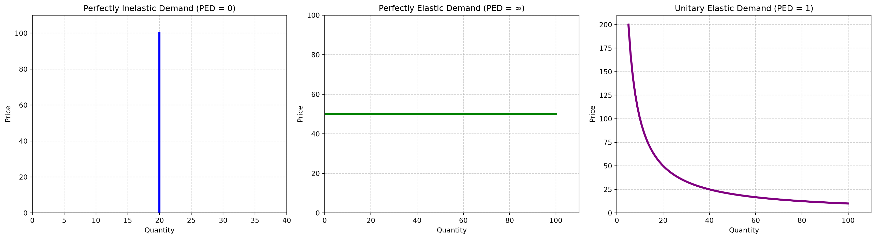
Perfectly Inelastic Demand ($\text{PED} = 0$): Quantity demanded is completely unresponsive to price changes (e.g., life-saving drugs like insulin). Graphically represented as a vertical line ($Q = k$) parallel to the $Y$-axis.
Perfectly Elastic Demand ($\text{PED} = \infty$): Consumers buy infinitely at a single specific price, but demand drops to zero at any higher price. Graphically represented as a horizontal line ($P = k$) parallel to the $X$-axis.
Unitary Elastic Demand Curve ($\text{PED} = 1.0$ throughout): Percentage change in quantity demanded exactly equals percentage change in price at all points. Graphically represented as a rectangular hyperbola ($P \times Q = k$).

Code

import matplotlib.pyplot as plt
import numpy as np

fig, axs = plt.subplots(1, 3, figsize=(18, 5))

# 1. Perfectly Inelastic Demand (PED = 0)
q_inelastic = [20, 20]
p_inelastic = [0, 100]
axs[0].plot(q_inelastic, p_inelastic, color='blue', lw=3)
axs[0].set_title('Perfectly Inelastic Demand (PED = 0)')
axs[0].set_xlabel('Quantity')
axs[0].set_ylabel('Price')
axs[0].set_xlim(0, 40)
axs[0].set_ylim(0, 110)
axs[0].grid(True, linestyle='--', alpha=0.6)

# 2. Perfectly Elastic Demand (PED = infinity)
q_elastic = [0, 100]
p_elastic = [50, 50]
axs[1].plot(q_elastic, p_elastic, color='green', lw=3)
axs[1].set_title('Perfectly Elastic Demand (PED = $\infty$)')
axs[1].set_xlabel('Quantity')
axs[1].set_ylabel('Price')
axs[1].set_xlim(0, 110)
axs[1].set_ylim(0, 100)
axs[1].grid(True, linestyle='--', alpha=0.6)

# 3. Unitary Elastic Demand (PED = 1)
# P * Q = k => P = k / Q
q_unitary = np.linspace(5, 100, 100)
k = 1000
p_unitary = k / q_unitary
axs[2].plot(q_unitary, p_unitary, color='purple', lw=3)
axs[2].set_title('Unitary Elastic Demand (PED = 1)')
axs[2].set_xlabel('Quantity')
axs[2].set_ylabel('Price')
axs[2].set_xlim(0, 110)
axs[2].set_ylim(0, 210)
axs[2].grid(True, linestyle='--', alpha=0.6)

plt.tight_layout()
plt.show()

<>:21: SyntaxWarning: "\i" is an invalid escape sequence. Such sequences will not work in the future. Did you mean "\\i"? A raw string is also an option.
<>:21: SyntaxWarning: "\i" is an invalid escape sequence. Such sequences will not work in the future. Did you mean "\\i"? A raw string is also an option.
C:\Users\Venu\AppData\Local\Temp\ipykernel_17384\3119259408.py:21: SyntaxWarning: "\i" is an invalid escape sequence. Such sequences will not work in the future. Did you mean "\\i"? A raw string is also an option.
  axs[1].set_title('Perfectly Elastic Demand (PED = $\infty$)')

2.2 Income Elasticity of Demand (YED)

2.2.1 Definition and Formula

Income Elasticity of Demand ($\text{YED}$ or $y$) measures the responsiveness of quantity demanded to changes in consumer income.

\[\text{YED} = \frac{\% \Delta Q_d}{\% \Delta Y} = \frac{\Delta Q}{\Delta Y} \times \frac{Y_1}{Q_1}\]

2.2.2 Good Classifications via YED

Normal Goods ($\text{YED} > 0$): Quantity demanded increases as consumer income rises.
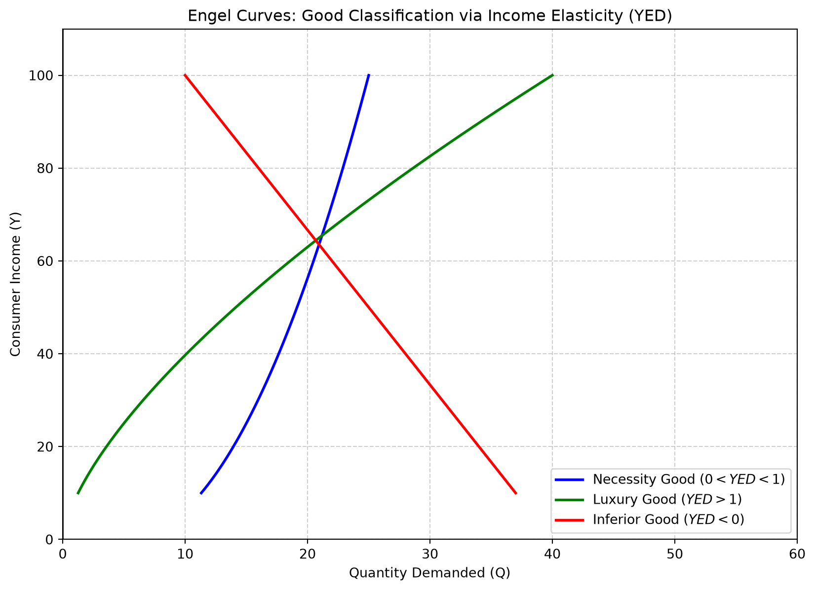
- Necessity Goods ($0 < \text{YED} < 1$): Quantity demanded increases by a smaller proportion than the increase in income (e.g., basic flour, rice, pulses).
- Luxury or Superior Goods ($\text{YED} > 1$): Quantity demanded increases by a greater proportion than the increase in income (e.g., designer clothing, jewelry, high-end electronics, premium dining/ramen, automobiles in developing economies).
Inferior Goods ($\text{YED} < 0$): Quantity demanded decreases as consumer income rises (e.g., low-grade cooking oil, cheap packet noodles like Maggi, lower-quality grain).

2.2.2.1 Graphing Conventions for YED

When plotting $\text{YED}$, Income ($Y$) is placed on the $Y$-axis and Quantity ($Q$) on the $X$-axis. Necessity curves are steep (closer to the $Y$-axis), Luxury curves are flat/gradual, and Inferior good curves bend backward (negative slope).

Code

import matplotlib.pyplot as plt
import numpy as np

# Income range
Y = np.linspace(10, 100, 100)

# 1. Necessity Good (0 < YED < 1) - Q increases slowly with Y
Q_necessity = 2 * np.sqrt(Y) + 5

# 2. Luxury Good (YED > 1) - Q increases rapidly with Y
Q_luxury = (Y**1.5) / 25

# 3. Inferior Good (YED < 0) - Q decreases as Y increases
Q_inferior = 40 - 0.3 * Y

plt.figure(figsize=(10, 7))

plt.plot(Q_necessity, Y, label='Necessity Good ($0 < YED < 1$)', color='blue', lw=2)
plt.plot(Q_luxury, Y, label='Luxury Good ($YED > 1$)', color='green', lw=2)
plt.plot(Q_inferior, Y, label='Inferior Good ($YED < 0$)', color='red', lw=2)

plt.title('Engel Curves: Good Classification via Income Elasticity (YED)')
plt.xlabel('Quantity Demanded (Q)')
plt.ylabel('Consumer Income (Y)')
plt.axvline(0, color='black', lw=1)
plt.axhline(0, color='black', lw=1)
plt.grid(True, linestyle='--', alpha=0.6)
plt.legend()
plt.xlim(0, 60)
plt.ylim(0, 110)

plt.show()

2.3 Cross-Price Elasticity of Demand (XED)

2.3.1 Definition and Formula

Cross-Price Elasticity of Demand ($\text{XED}$) measures the responsiveness of quantity demanded of Product $A$ following a change in the price of Product $B$.

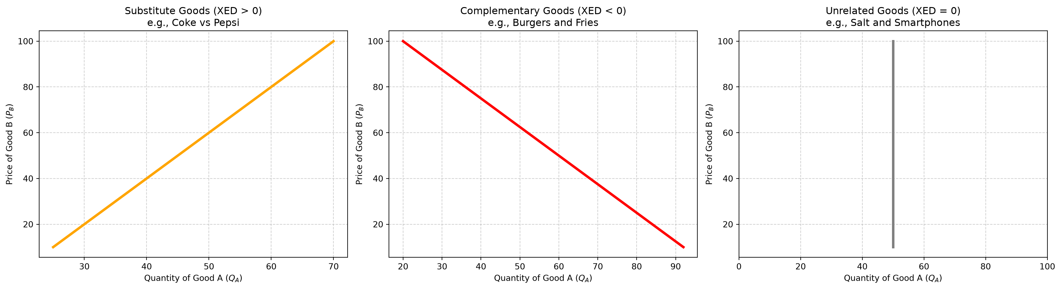
\[\text{XED}_{AB} = \frac{\% \Delta Q_A}{\% \Delta P_B} = \frac{\Delta Q_A}{\Delta P_B} \times \frac{P_{B1}}{Q_{A1}}\]

2.3.2 Good Relationships via XED

Substitute Goods ($\text{XED} > 0$): A price increase for Product $B$ increases demand for Product $A$ as consumers switch products (e.g., Coca-Cola vs. Pepsi, PCs vs. Laptops, a la carte vs. set meals).
Complementary Goods ($\text{XED} < 0$): A price increase for Product $B$ reduces demand for Product $A$ as the goods are consumed jointly (e.g., cinema tickets and popcorn, petrol and cars, smartphone contracts and mobile apps).
Unrelated Goods ($\text{XED} = 0$): Changes in the price of one product have no effect on the demand for the other.

Code

import matplotlib.pyplot as plt
import numpy as np

fig, axs = plt.subplots(1, 3, figsize=(18, 5))

# 1. Substitutes (XED > 0)
pb_sub = np.linspace(10, 100, 100)
qa_sub = 20 + 0.5 * pb_sub
axs[0].plot(qa_sub, pb_sub, color='orange', lw=3)
axs[0].set_title('Substitute Goods (XED > 0)\ne.g., Coke vs Pepsi')
axs[0].set_xlabel('Quantity of Good A ($Q_A$)')
axs[0].set_ylabel('Price of Good B ($P_B$)')
axs[0].grid(True, linestyle='--', alpha=0.6)

# 2. Complements (XED < 0)
pb_comp = np.linspace(10, 100, 100)
qa_comp = 100 - 0.8 * pb_comp
axs[1].plot(qa_comp, pb_comp, color='red', lw=3)
axs[1].set_title('Complementary Goods (XED < 0)\ne.g., Burgers and Fries')
axs[1].set_xlabel('Quantity of Good A ($Q_A$)')
axs[1].set_ylabel('Price of Good B ($P_B$)')
axs[1].grid(True, linestyle='--', alpha=0.6)

# 3. Unrelated Goods (XED = 0)
pb_unrel = np.linspace(10, 100, 100)
qa_unrel = np.full_like(pb_unrel, 50)
axs[2].plot(qa_unrel, pb_unrel, color='gray', lw=3)
axs[2].set_title('Unrelated Goods (XED = 0)\ne.g., Salt and Smartphones')
axs[2].set_xlabel('Quantity of Good A ($Q_A$)')
axs[2].set_ylabel('Price of Good B ($P_B$)')
axs[2].set_xlim(0, 100)
axs[2].grid(True, linestyle='--', alpha=0.6)

plt.tight_layout()
plt.show()

3 Operational Dynamics and Impact on Decision-Making

3.1 Determinants of Price Elasticity of Demand

Availability and Attractiveness of Substitutes: Goods with close, attractive substitutes (e.g., filter coffee vs. Nescafe, KFC vs. 5-Star Chicken) have highly elastic demand.
Relative Expense as a Proportion of Income: Products accounting for a small fraction of a consumer’s budget (e.g., a cup of coffee) have lower $\text{PED}$, whereas large budget items (e.g., housing rent) exhibit higher $\text{PED}$ over time.
Time Horizon: Demand is less elastic in the short run because spending habits take time to alter, but becomes increasingly elastic in the long run as consumers locate substitutes.

3.2 The Total Revenue / Total Spending Test

Total Revenue ($\text{TR}$) or Total Spending is defined as $\text{TR} = P \times Q$. - Unitary Elastic Demand ($\text{PED} = 1.0$): A price change causes an exact offset in quantity demanded, leaving total spending completely unchanged ($\% \Delta P = \% \Delta Q_d$). - Price Inelastic Demand ($\text{PED} < 1.0$): A price increase results in a smaller percentage drop in quantity demanded ($\% \Delta P > \% \Delta Q_d$), increasing total revenue. - Price Elastic Demand ($\text{PED} > 1.0$): A price increase results in a larger percentage drop in quantity demanded ($\% \Delta Q_d > \% \Delta P$), decreasing total revenue.

3.3 Producer and Consumer Applications

Pricing and Retail Channels: Manufacturers adjust prices based on channel-specific elasticity (e.g., local market stalls with $\text{PED} = 1.0$, fashion boutiques with inelastic $\text{PED} = 0.5$, and online shops with highly elastic $\text{PED} = 3.0$ due to instant price comparison).
Taxation and Subsidies: Governments evaluate $\text{PED}$ to predict tax yields or subsidy efficiency.
Resource Reallocation Across Competitor Goods: When two goods share the same resource base in an industry (e.g., leaf tea vs. dust tea, sedans vs. SUVs), a drop in the price of one competitor good reduces its profitability, prompting producers to redeploy resources to increase the supply of the other good.

4 Real-Life Case Studies from Class Discussions

4.1 Case Study 1: Global Coffee Market Mechanization

Context: Global coffee prices dropped to a 13-year low, severe for Brazilian and Indian growers.
Mechanization Drive: Producers introduced $150,000 harvesting machines cutting harvest costs by 40–60%.
Market Paradox: Despite rising global coffee demand, prices crashed because supply growth outpaced demand growth due to rapid mechanization.
Ethical & Structural Issues: Mechanization made rural plantation labor redundant, driving rural unemployment. Non-perishable coffee stockpiles in godowns created a multi-year supply overhang preventing price recovery.

4.2 Case Study 2: Restaurant Demand Analysis (Chicken and Rice Meal)

Problem: A restaurant raised chicken meal prices and observed a drop in orders.
Competing Hypotheses & Diagnostic Data Needed:
- Elasticity Measurements: Exact price change vs. order drop size.
- Menu Substitutes: Cross-substitution toward mutton/fish dishes or ala carte options.
- External Substitutes: Nearby competing restaurants within 0.5 km.
- Customer Income & Population Drifts: Local economic downturns or conversions of family housing into student/bachelor hostels.
- Complements & Combos: Removal of complementary free drinks or bundled combo offers.
- Exogenous Factors: Ingredient/chef changes, bird flu health scares, seasonal school terms, or deteriorating store ambience/drainage issues.

4.3 Case Study 3: Natural Gas & Energy Policy in China

Data Provided: Short-run $\text{PED} = -1.52$, Long-run $\text{PED} = +0.41$ (identified as a printing typo and corrected to $-0.41$). $\text{XED}$ of coal with respect to natural gas prices was $-0.76$ (short run) and $+0.01$ (long run).
Policy Analysis: A $10\%$ reduction in natural gas prices increases natural gas consumption by $15.2\%$ in the short run. Simultaneously, it reduces coal demand by $7.6\%$. Economists use these elasticities to design taxes on coal and oil to accelerate green energy adoption.

4.4 Case Study 4: Fidget Spinner Market Shifters

Classroom Learning Study Finding: Tastes/preferences shift $\implies$ Demand curve shifts Right.
Bearing Resource Price Increase: Input costs rise $\implies$ Supply curve shifts Left.
Fidget Cube Substitute Price Drop: Substitute cheaper $\implies$ Demand for fidget spinners shifts Left.
Fidget Spinner Price Drop: Own-price change $\implies$ Movement along curve (Quantity Demanded rises).
Government Producer Subsidy: Cost reduction $\implies$ Supply curve shifts Right.
Recession / Income Fall: Incomes drop for normal good $\implies$ Demand curve shifts Left.
Complement Price Drop: Complement cheaper $\implies$ Demand curve shifts Right.
Simultaneous Demand and Supply Increase: Quantity increases unambiguously; Price outcome is indeterminate.

5 Textbook Questions and Exam Practice Solutions

Linear Demand Gradient: A straight-line demand curve has a constant gradient, meaning quantity changes in proportion to price changes.
Substitute Price Surge: A large price increase for iced tea causes consumers to switch, shifting the demand curve for cola to the right.
Individual Income Drop: A decrease in an individual’s income shifts their personal demand curve for a Range Rover Evoke to the left.
Production Worker Wage Increase: Higher labor costs shift the market supply curve for Range Rovers to the left.
Cooking Oil Subsidy: Government subsidies lower production costs, shifting the market supply curve to the right.
Tax on Imported US Orange Juice: Import taxes reduce raw material availability/imported supply, shifting the domestic orange juice market supply curve to the left.
Calculated Tourism Cross-Elasticity: Australian tourists visiting Indonesia relative to Malaysian trip prices ($\text{XED} = 2.4$). A $5\%$ increase in Malaysian trip prices yields a $2.4 \times 5\% = 12\%$ surge in Indonesian visits.
Promotional Product Selection: When selecting products for promotion under rising consumer incomes, goods with high positive $\text{YED}$ will expand naturally; promotional efforts/discounts should target products hardest hit by rising incomes or those with high $\text{PED}$ (e.g., Product $D$ with $\text{PED} = 2.0, \text{YED} = -1.7$).