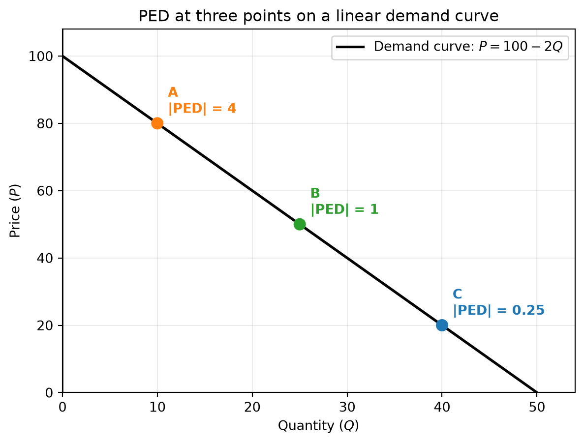
PED Changes - Linear Demand Curve
Definition of Price Elasticity of Demand (PED)
Price elasticity of demand (PED) measures the responsiveness of the quantity demanded of a good to a change in its price.
Formally:
\[ \text{PED} = \frac{\%\ \text{change in quantity demanded}}{\%\ \text{change in price}} \]
or, using calculus for a demand function \(Q = f(P)\):
\[ \text{PED} = \frac{dQ}{dP} \times \frac{P}{Q} \]
Key points:
- PED is usually negative for normal goods (because of the law of demand), but we often refer to its absolute value \(|\text{PED}|\).
- Interpretation:
- \(|\text{PED}| > 1\): Elastic demand (quantity responds strongly to price changes).
- \(|\text{PED}| = 1\): Unitary elastic demand.
- \(|\text{PED}| < 1\): Inelastic demand (quantity responds weakly to price changes).
How PED Changes Along a Straight-Line Demand Curve
On a typical downward-sloping straight-line (linear) demand curve, PED is not constant:
- High prices / low quantities (upper part of the curve): demand is more elastic.
- Midpoint of the curve: demand is unitary elastic (\(|\text{PED}| = 1\)).
- Low prices / high quantities (lower part of the curve): demand is more inelastic.
Why PED changes even though the slope is constant
For a linear demand curve, the slope \(\frac{dP}{dQ}\) (or \(\frac{dQ}{dP}\)) is constant, but PED depends on both the slope and the ratio \(\frac{P}{Q}\):
\[ \text{PED} = \frac{dQ}{dP} \times \frac{P}{Q} \]
- \(\frac{dQ}{dP}\) is constant for a straight line.
- But \(\frac{P}{Q}\) changes as you move along the curve.
So even with a constant slope, the percentage responsiveness changes because the base levels of \(P\) and \(Q\) change.
Intuitively:
- At the top-left (high \(P\), low \(Q\)): a given absolute change in price is a small percentage change, but the same absolute change in quantity is a large percentage change → high elasticity.
- At the bottom-right (low \(P\), high \(Q\)): the same absolute price change is a large percentage change, but the quantity change is a small percentage change → low elasticity.
Numerical Example
Consider a simple linear demand function:
\[ P = 100 - 2Q \quad \text{or} \quad Q = 50 - 0.5P \]
Here, \(\frac{dQ}{dP} = -0.5\) (constant).
PED at any point:
\[ \text{PED} = \frac{dQ}{dP} \times \frac{P}{Q} = -0.5 \times \frac{P}{Q} \]
Point A: High price, low quantity (elastic region)
Let \(Q = 10\):
- \(P = 100 - 2(10) = 80\)
- \(\text{PED} = -0.5 \times \frac{80}{10} = -0.5 \times 8 = -4\)
\(|\text{PED}| = 4 > 1\) → elastic demand.
Point B: Midpoint (unitary elasticity)
Midpoint in quantity terms: \(Q = 25\)
- \(P = 100 - 2(25) = 50\)
- \(\text{PED} = -0.5 \times \frac{50}{25} = -0.5 \times 2 = -1\)
\(|\text{PED}| = 1\) → unitary elastic.
Point C: Low price, high quantity (inelastic region)
Let \(Q = 40\):
- \(P = 100 - 2(40) = 20\)
- \(\text{PED} = -0.5 \times \frac{20}{40} = -0.5 \times 0.5 = -0.25\)
\(|\text{PED}| = 0.25 < 1\) → inelastic demand.
So along the same straight line:
- Top segment: \(|\text{PED}| > 1\) (elastic)
- Midpoint: \(|\text{PED}| = 1\) (unitary)
- Bottom segment: \(|\text{PED}| < 1\) (inelastic)
Explaining PED = 1 at the mid point
Another way of calculating PED is that on a demand curve,
\(\text{PED} = \text{Lower Segment} / \text{Upper Segment}\)
Let us see how this can be derived.
The Starting Point: The Elasticity Formula
The standard point elasticity of demand formula is: \[\text{PED} = \frac{\% \Delta Q}{\% \Delta P} = \frac{dQ}{dP} \times \frac{P}{Q}\] On a standard graph:
- Price (\(P\)) is on the vertical axis (Y-axis).
- Quantity (\(Q\)) is on the horizontal axis (X-axis).
Because the axes are flipped relative to typical math conventions (\(P\) is independent but on the Y-axis), the mathematical slope of the demand curve is \(\frac{dP}{dQ}\). Therefore, \(\frac{dQ}{dP}\) is actually \(\frac{1}{\text{slope}}\) of the demand curve.
Setting up the Geometry
Imagine a straight-line demand curve that intersects the vertical Price axis at point \(A\) and the horizontal Quantity axis at point \(B\). Let’s pick any random point \(C\) on this demand curve to measure elasticity:
- Draw a horizontal line from \(C\) to the Price axis; call this point \(P_c\) (this represents the current Price).
- Draw a vertical line from \(C\) down to the Quantity axis; call this point \(Q_c\) (this represents the current Quantity).
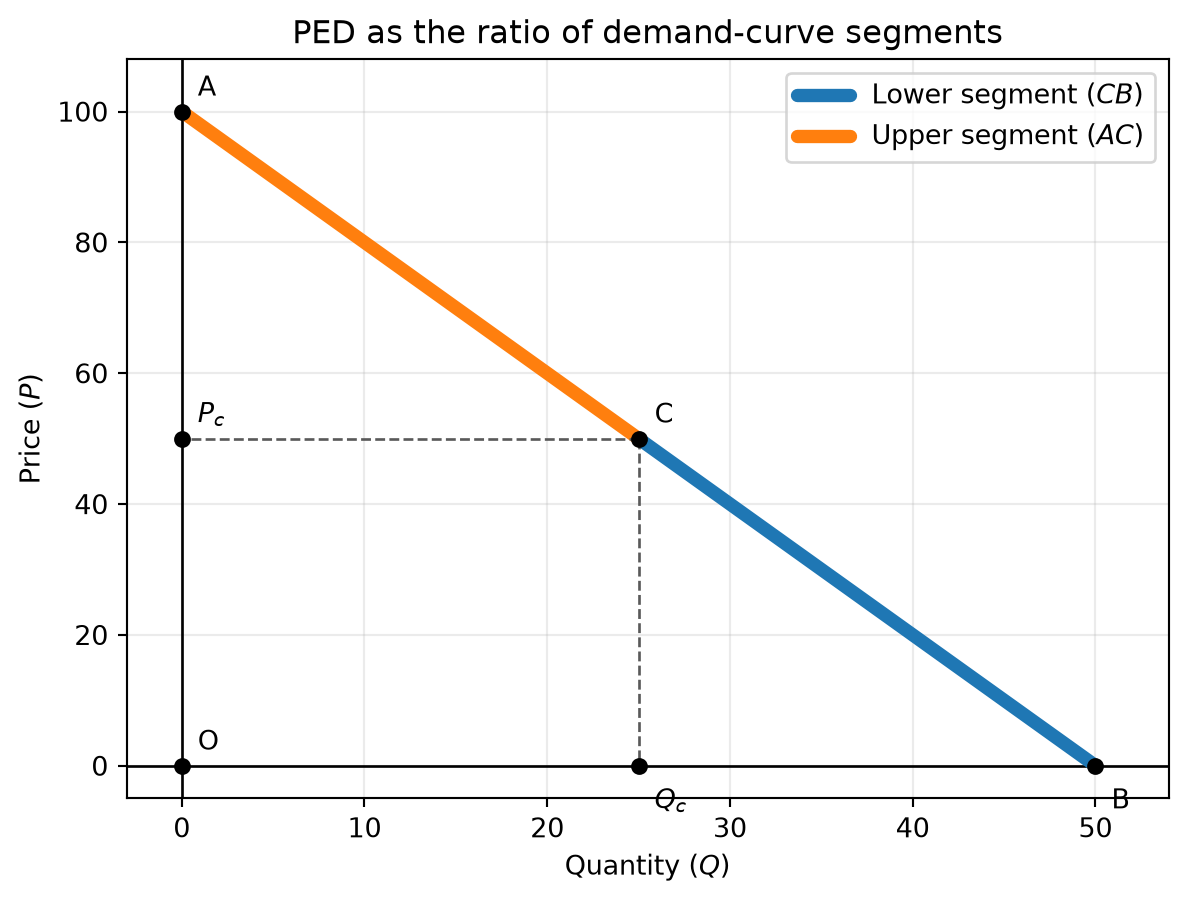
Notice the Similar Triangles
By dropping these lines, we create a series of similar triangles (triangles that have the exact same angles but different sizes):
- The top triangle: \(\triangle A P_c C\)
- The bottom triangle: \(\triangle C Q_c B\)
Because these triangles are similar, the ratios of their corresponding sides must be exactly equal.
Let’s look at the components of our elasticity formula (\(\frac{1}{\text{slope}} \times \frac{P}{Q}\)):
\(\frac{1}{\text{slope}}\) (which is \(\frac{\Delta Q}{\Delta P}\)) can be represented by the base and height of the lower triangle: \(\frac{Q_c B}{C Q_c}\).
\(\frac{P}{Q}\) is the price at point \(C\) divided by the quantity at point \(C\), which matches the lengths \(\frac{C Q_c}{O Q_c}\) (where \(O\) is the origin).
When you multiply them together: \[\text{PED} = \left(\frac{Q_c B}{C Q_c}\right) \times \left(\frac{C Q_c}{O Q_c}\right)\] Notice that \(C Q_c\) appears on both the top and the bottom, so they cancel each other out: \[\text{PED} = \frac{Q_c B}{O Q_c}\]
Relating to the Hypotenuse (The Segments)
Because \(\triangle A P_c C\) and \(\triangle C Q_c B\) are similar, the ratio of their horizontal bases (\(\frac{Q_c B}{O Q_c}\)) is perfectly identical to the ratio of their hypotenuses along the demand curve itself.
- The line segment \(C B\) represents the Lower Segment (from point \(C\) down to the Quantity axis).
- The line segment \(A C\) represents the Upper Segment (from the Price axis down to point \(C\)).
Therefore, by geometric substitution: \[\text{PED} = \frac{\text{Distance from } C \text{ to } B}{\text{Distance from } A \text{ to } C} = \frac{\text{Lower Segment}}{\text{Upper Segment}}\] ——————————
Visualizing the Result
This geometric approach gives us another way of thinking about elasticity along the demand curve.
At the Price Intercept (Top): The lower segment is the entire line, and the upper segment is zero. \(\text{PED} = \text{Length} / 0 = \infty\) (Perfecty Elastic).
At the Midpoint: The lower segment exactly equals the upper segment. \(\text{PED} = 1 / 1 = 1\) (Unitary Elastic).
At the Quantity Intercept (Bottom): The lower segment is zero, and the upper segment is the entire line. \(\text{PED} = 0 / \text{Length} = 0\) (Perfecty Inelastic).
Key Pattern to Remember (for Exams)
On a typical downward-sloping straight-line demand curve:
- Upper half: \(|\text{PED}| > 1\) → elastic
- Midpoint: \(|\text{PED}| = 1\) → unitary
- Lower half: \(|\text{PED}| < 1\) → inelastic
- At the price-axis intercept (where \(Q = 0\)): \(|\text{PED}| \to \infty\) (perfectly elastic in the limit)
- At the quantity-axis intercept (where \(P = 0\)): \(\text{PED} = 0\) (perfectly inelastic in the limit)